Expectation Maximization

EM is the algorithm you reach for when maximum likelihood is clear in principle but hard in practice because of latent variables. Gaussian mixtures are the canonical example.

This post keeps one thread: define the mixture objective, split optimization into E and M steps, and explain why each subproblem is easier than direct optimization of the marginal likelihood.

As in the previous post, in a Gaussian mixture model we maximize likelihood over means, covariances, and mixing weights.

Intuitively, EM alternates between two questions: given parameters, which cluster likely generated each point (E-step)? Given those soft assignments, what parameters best fit them (M-step)?

1. Initialize the means $\mu_k$, covariances $\Sigma_k$ and mixing coefficients $\pi_k$ , and evaluate the initial value of the log likelihood.
2. E step: Evaluate the responsibilities using the current parameter values.

$$ \begin{aligned} \gamma(z_k) = & p(z_k=1|x) \\\ = & \frac{p(z_k=1).p(x|z_k=1)}{\sum_{j=1}^Kp(z_j=1).p(x|z_j=1)} \\\ =& \frac{\pi_k.\text{Normal}(x|\mu_k,\Sigma_k)}{\sum_{j=1}^K\pi_j.\text{Normal}(x|\mu_j,\Sigma_j)} \end{aligned} $$

3. M step: Re-estimate the parameters using the current responsibilities. Where we saw that to find a minimizer, set the gradient to $0$: $$ \begin{aligned} \mu_k = \frac{1}{N_k} \sum_{n=1}^N \gamma(z_{nk})x_n \end{aligned} $$ which is weighted average data points where $N_k = \sum_{n=1}^N \gamma (z_{nk})$ is efficient number of data points assigned to cluster $k$.

4. Similarly, if we fix $\mu,\pi$ we can optimize over $\Sigma$:

$$ \begin{aligned} \Sigma_k = \frac{1}{N_k} \sum_{n=1}^N \gamma(z_{nk})(x_n-\mu_k)(x_n-\mu_k)^T \end{aligned} $$

5. If we fix $\mu,\Sigma$ we can then optimize over $\pi$:

$$ \pi_k = \frac{N_k}{N} $$

6. Evaluate the log-likelihood and check for convergence of either the parameters or the log-likelihood. If the convergence criterion is not satisfied, return to step 2: $$ p(X|\mu,\Sigma,\pi) = \sum_{n=1}^N \ln \left\{ \sum_{k=1}^K \pi_k . \text{Normal}(x_n|\mu_k,\Sigma_k) \right\} $$

Now, let’s talk about a few basic concepts:

Mixture models (latent variable model)

Suppose we have a probabilistic model: $$ p(x,z| \theta) $$

Where:

1. $x$: observed data
2. $z$: hidden/latent variable $z\in \{ 1,..,K\}$ and $p(z=k)=\pi_k$ and $p(x|z) = \text{Normal}(\mu_k,\Sigma_k)$
3. $\theta$: parameter

Marginal on $x$ is defined as: $$ p(x|\theta) = \sum_z p(x,z|\theta) $$

Direct optimization of $p(x|\theta)$ is often tricky, but we can optimize complete data likelihood $p(x,z|\theta)$. We use EM algorithm to approximate $\max_{\theta} p(x|\theta)$ by repeating two steps:

1. E step (Expectation step)
2. M step (Maximization step)

Which are easier to implement.

Review: a function $f: \mathbb{R} \rightarrow \mathbb{R}$ is convex if $f’’(x)\geq 0$ for all $x \in \mathbb{R}$.

The curve below illustrates convexity: line segments between points stay above the function.

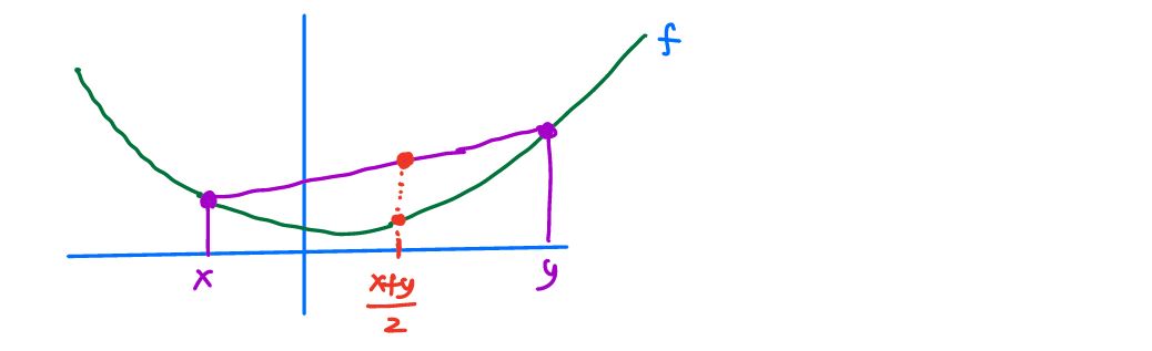
Equivalently we can say:

$$ f(\frac{x+y}{2}) \leq \frac{f(x)+f(y)}{2} $$

We can write this down with the following equation (i.e., the previous one holds for $n=1$ and $\lambda_1=\lambda_2=\frac{1}{2}$):

$$ f(\sum_{i=1}^n \lambda_i x_i) \leq \sum_{i=1}^n \lambda_i f(x_i) $$

for all $x_1,..,x_n \in \mathbb{R}$ and $\lambda_1,..,\lambda_n \geq 0$ and $\sum_{i=1}^n \lambda_i = 1$.

Based on Jensen’s inequality for all random variable $x$ (i.e., in our example the distribution of $x$ is $\sum_{i=1}^n \lambda_i \delta_{x_i}$):

$$ f(\mathbb{E}[x]) \leq \mathbb{E}[f(x)] $$

MLE for $\theta$

Let’s say we want to find $\max_{\theta} \log p(x|\theta)$. Log-likelihood has summation inside logarithm: $$ L(\theta) = \log p(x|\theta) = \log \sum_{z} p(x,z| \theta) $$

Idea: is to introduce an auxiliary distribution $q(z)$ over $z$ (i.e., $q(z) > 0 , \sum_z q(z)=1$). Then we can lower bound the log-likelihood:

$$ \begin{aligned} \log p(x| \theta) = & \log \sum_z p(x,z| \theta) \\ =& \log \sum_z \frac{q(z)}{q(z)} p(x,z| \theta) \\ = & \log \sum_z q(z) \frac{p(x,z|\theta)}{q(z)} \\ = & \log \mathbb{E}_{z\sim q} \left[ \frac{p(x,z| \theta)}{q(z)}\right] \end{aligned} $$

Then we can say:

$$ \log p(x|\theta) \geq \mathbb{E}_{z\sim q} \left[ \log \frac{p(x,z| \theta)}{q(z)}\right] $$

which is derived from the Jensen’s inequality for:

$$ f(x) = -\log x $$

Which is not linear. This function is convex because: $$ \begin{aligned} f’(x) = - \frac{1}{x} \\ f’’(x) = \frac{1}{x^2} \end{aligned} $$

Then by Jensen’s inequality for any random variable $Y$: $$ \begin{aligned} f(\mathbb{E}[Y]) \leq & \mathbb{E}[f(Y)] \\ -\log \mathbb{E}[Y] \leq & \mathbb{E}[-\log Y] \\ \mathbb{E}[\log Y] \leq & \log \mathbb{E}[Y] \end{aligned} $$

For example if we take $Y=\frac{p(x,z|\theta)}{q(z)}$ with $z\sim q$, we can say:

$$ \mathbb{E}[\log \frac{p(x,z|\theta)}{q(z)}] \leq \log \mathbb{E}_q[\frac{p(x,z|\theta)}{q(z)}] $$

Therefore, for any distribution, we have a lower bound: $$ \log p(x|\theta) \geq \text{ELBO}(x,q|\theta) $$

where ELBO (evidence lower bound ) is $$ \text{ELBO}(x,q|\theta) = \sum_z q(z) \log \frac{p(x,z|\theta)}{q(z)} $$

So the question is, what is the best distribution $q$? When do we have equality in Jensen’s inequality ? In general, inequality: $$ f(\mathbb{E}[x]) \leq \mathbb{E}[f(x)] $$

becomes equality (i.e., $f(\mathbb{E}[x]) = \mathbb{E}[f(x)]$) if:

1. $f(x)$ is linear
2. $Y$ is a constant random variable.

As discussed earlier, the function $f(x)= -\log x$ is not linear. Then, it has to be a constant:

$$ Y = \frac{p(x,z|\theta)}{q(z)} $$

which means $q(z) \propto p(x,z|\theta)$ over $z$. Since $q(z)$ is a distribution, $\sum_z q(z) =1$. Then, we must have the following:

$$ q(z) = \frac{p(x,z|\theta)}{\sum_{z’}p(x,z’|\theta)} = \frac{p(x,z|\theta)}{p(x|\theta)} = p(z|x,\theta) $$

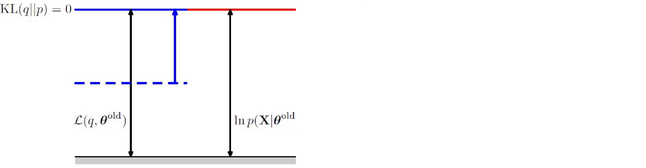
E step: $q(z) = p(z|x,\theta)$ then we have equality in bound: $$ \log p(x|\theta) = \text{ELBO}(x,q|\theta) $$

when $q(z) = p(z|x,\theta^{\text{old}})$ then: $$ \begin{aligned} \text{ELBO}(x,q|\theta)= & \sum_z q(z) \log \frac{p(x,z|\theta)}{q(z)} \\ = & \sum_z p(z|x,\theta^{\text{old}}) \log p(x,z|\theta) - \sum_z q(z) \log q(z) \\ = & Q(\theta,\theta^{\text{old}}) + \text{Entropy}(q) \\ = & Q(\theta,\theta^{\text{old}}) + c \end{aligned} $$

then we can update $\theta$ by:

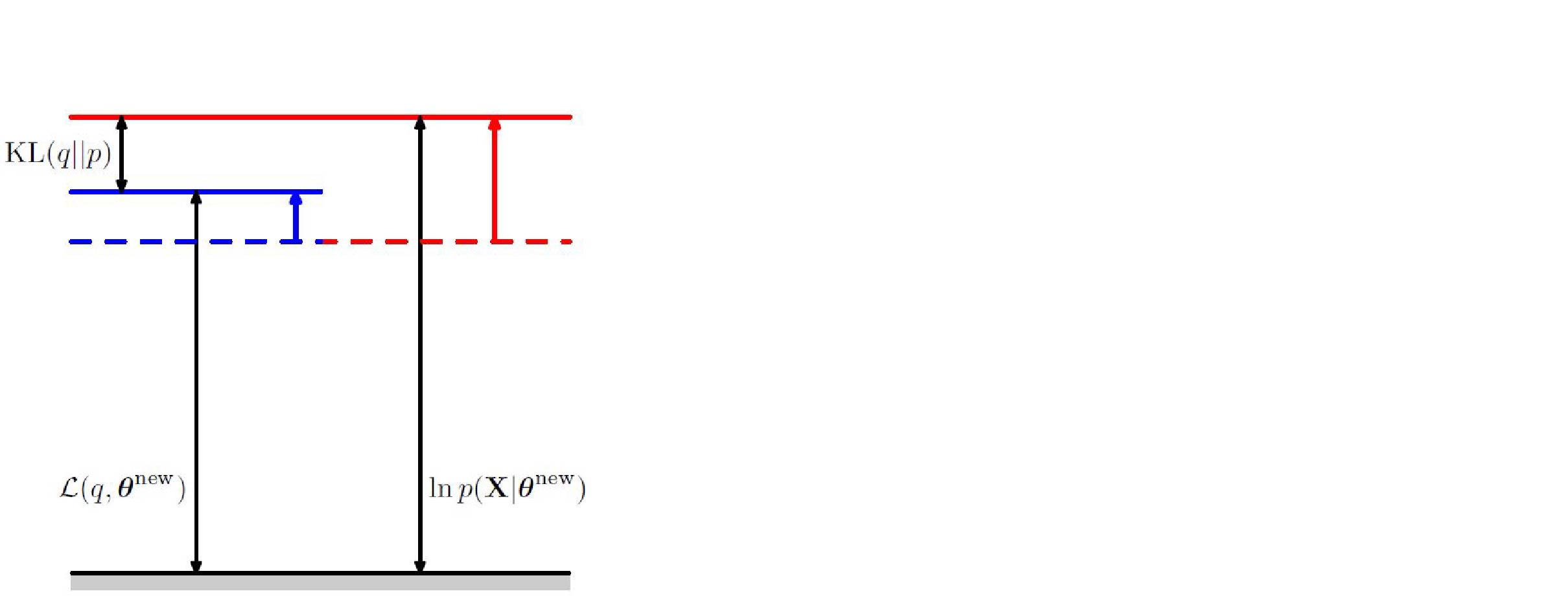
M Step: $$ \theta^{\text{new}} = \arg \max_{\theta} Q(\theta,\theta^{\text{old}}) $$

where $Q(\theta,\theta^{\text{old}}) = \sum_z p(z| x,\theta^{\text{old}}) \log p(x,z|\theta)$.

EM algorithm converges to local maxima because each step improves log-likelihood: $$ \log p(x|\theta^{\text{new}}) \geq \log p(x|\theta^{\text{old}}) $$

Because:

$$ \begin{aligned} \log p(x|\theta^{\text{new}}) \geq & \text{ELBO} (x,q| \theta^{\text{new}}),(\text{i.e., } q = p(z| x,\theta^{\text{old}})) \\ \geq & \text{ELBO}(x,q|\theta^{\text{old}}), (\text{bc }\theta^{\text{new}} = \arg \max_{\theta} Q(\theta,\theta^{\text{old}})) \\ =& \log p(x|\theta^{\text{old}}) \end{aligned} $$

As you see, EM is an iterative method to maximize $\log p(x|\theta)$ and may converge to local maxima. We may need to run multiple times.

We also have the following decomposition:

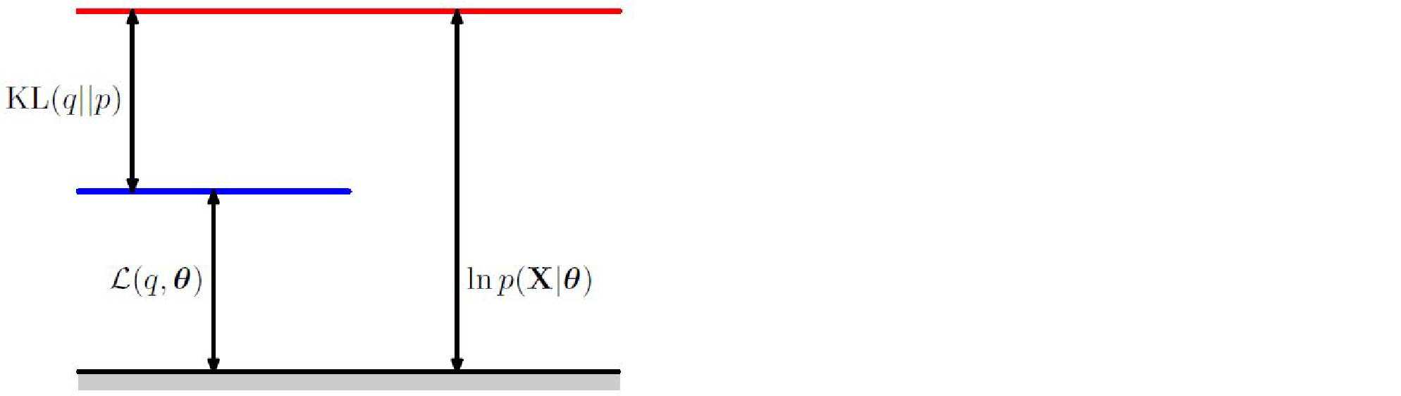
$$ \text{ELBO}(x,q|\theta) = \mathcal{L}(q,\theta) = \log p(x|\theta) - \text{KL}(q || p(z|x,\theta)) $$

where $\text{KL}(q || p(z|x,\theta)) = \sum_z q(z)\log \frac{q(z)}{p(z|x,\theta)}$.

1. Since $\text{KL} \geq 0 $ then $\text{ELBO}(x,q|\theta)\leq \log p(x|\theta)$.
2. $\text{ELBO}(x,q|\theta) = \log p(x|\theta)$ if $\text{KL}(q || p(z|x,\theta))=0$, which holds if and only if $q(z) = p(z|x,\theta)$.

In general, for any distributions $q(z)$ and $p(z)$, the Kullback-Leibler divergence of $q$ with respect to $p$ is:

$$ \text{KL}(q || p) = \sum_z q(z) \log \frac{q(z)}{p(z)} $$

These Bishop figures summarize the geometric interpretation of the E-step:

and M-step:

and the decomposition:

Properties:

1. $\text{KL}(p || q) \geq 0 \quad \forall p,q$
2. $\text{KL}(p || q) = 0 \iff p=q$
3. $\text{KL}(p || q) \neq \text{KL}(q || p)$

We covered this post in the introduction to machine learning CPCS 481/581, Yale University, Andre Wibisono where I (joint with Siddharth Mitra) was TF.