Learning Optimal Transport from Samples

Optimal transport gives a principled way to match one distribution to another by minimizing movement cost, but high-dimensional settings make classic solvers expensive. This post focuses on that practical gap between elegant theory and scalable learning.

We use one roadmap: Monge and Kantorovich formulations, why direct computation becomes difficult, and how convex neural parameterizations (ICNNs) help learn transport maps from samples.

Throughout the post, source and target locations are denoted by $\alpha$ and $\beta$, while $a$ and $b$ denote their associated distributions. The main reference is Makkuva et al. (ICML 2020).

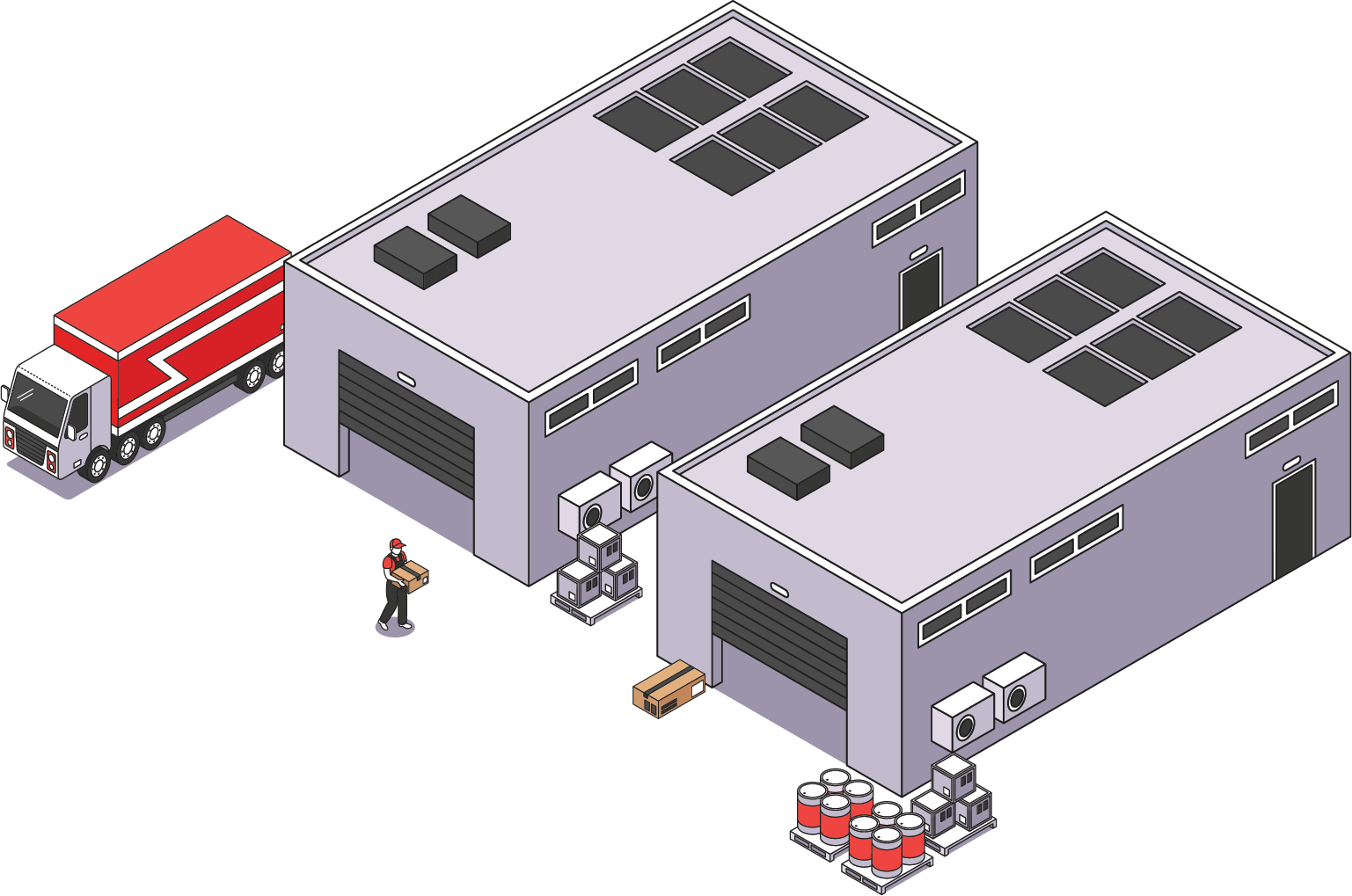
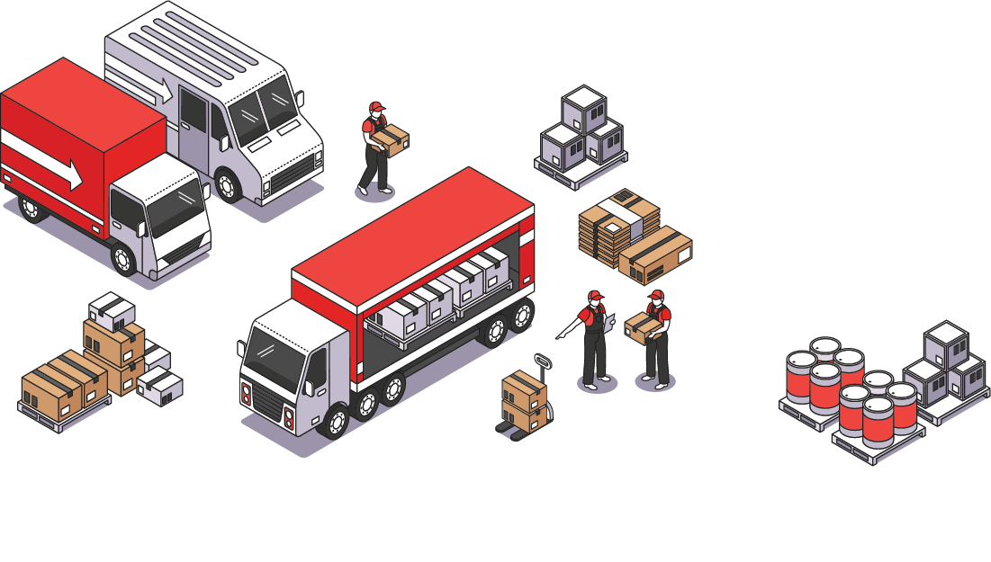
Historically, OT was motivated by logistics problems such as moving goods across locations at minimum cost.

The figure below illustrates that source-to-target transport intuition before we formalize it.

We’ll first discuss the Monge problem itself and then describe the sampling approach of Makkuva et al. to learn mappings.

Monge Problem

Let’s define resources $x_1,..,x_n$ in $\alpha$ and resources $y_1,..,y_m$ in $\beta$. We assign weight vectors $a$ and $b$ to these resources and define matrix $C$ as a measure of the pairwise distances between points $x_i \in \alpha$ and relative points derived from $T (x_i)$ in $\beta$. The Monge problem seeks to solve the following optimization problem:

$$ \min_{ T} \{ \sum_i C(x_i, T (x_i)) : T_{\sharp} \alpha = \beta \} $$

where the push-forward operator $\sharp$ represents the direction of the transportation plan.

Kantorovich Relaxation

Kantorovich proposed a relaxation of the Monge problem, allowing a source bin to be distributed to multiple locations in the target. Feasible solutions for this problem are defined by $U$ as follows:

$$ U(a,b) = \{T \in \mathrm{R}^{n\times m}_+ : T \mathrm{1}_m = a , T^T \mathrm{1}_n = b\}, $$

This ensures no particle or mass is lost during the transportation plan $T$ for vectors of all 1s and distributions $a$ and $b$. An optimal solution is obtained by solving the following problem for a given ground metric matrix $C \in \mathbb{R}^{n\times m}$: $$ L_c(a,b) = \min_{T \in U(a,b)} \langle C, T \rangle = \sum_{i,j} C_{i,j} T_{i,j}. $$

Linear Programming

With some linear algebra, we can formulate the Kantorovich relaxation as a linear programming problem:

$$ L_c(\alpha, \beta) = \min_{T} C^T T \text{ s.t., } A \underline{T} = \begin{bmatrix} \alpha \\ \beta \end{bmatrix} $$

where the matrix form is:

Algorithmic solutions for this linear program are well-established. In high-dimensional spaces, however, the proposed algorithms become computationally prohibitive. Some research has suggested quantizing space to handle the curse of dimensionality. For instance, a semi-discrete approach was proposed at ICML 2019 by the UIUC group.

1. If the source randomness of the network is a distribution, optimal transport can be achieved via deterministic evaluation.
2. For optimal transport mapping between a generator network and target distribution, the Wasserstein distance can be minimized through regression between generated data and mapped target points ($\Phi_1, \Phi_2,..,\Phi_N$): $$ L(x) = \frac{1}{B} \sum_{j=1}^B \min_i (c(x_j,y_i)-\Phi_i) + \frac{1}{N} \sum_{i=1}^N \Phi_i $$

This approach requires evaluating each point, and heuristic methods sample issues and use those as regularizers, potentially leading to biases. Makkuva et al. proposed learning optimal transport from samples by exploring convex function sets.

The next figure summarizes the convex-dual view used in the sample-based method.

Their method utilizes a dual form of Kantorovich’s relaxation:

$$ W(a,b) = \sup_{(f,g) \in \phi_c} \mathrm{E}_a[f(x)] + \mathrm{E}_b[g(y)] $$

where $\phi_c$ represents a set of constrained functions with $f(x) + g(y) \leq \frac{1}{2} ||x-y||^2$.

Input-Convex Neural Networks

Input-convex neural networks (ICNNs) are a class of neural networks where outputs are convex with respect to inputs, defined recursively by:

$$ f(x;\theta) = h_L \quad \text{where} \quad h_{l+1} = \sigma_l (W_l h_l + b_l + A_l x), \quad l = 0,1,..,L-1 $$

Based on this architecture, Makkuva et al. solve the Kantorovich dual problem using ICNNs, minimizing the need for new regularization.

$$ W(a,b) = C_{a,b} - \inf_{(f,g) \in \phi_c} \mathrm{E}_a[f(x)] + \mathrm{E}_b[g(y)] $$

where $C_{a,b} = \frac{1}{2} \mathrm{E}[x^2] + \frac{1}{2} \mathrm{E}[y^2]$, based on $f(x) + g(y) \leq \frac{1}{2} ||x-y||^2$.

Ultimately, we can define the optimal transport map $\nabla f^*$ by Brenier’s theorem:

$$ \mathrm{E}_b ||\nabla f^*(y)- y||^2 = \inf_{T: T_{\sharp} a = b} \mathrm{E}_b ||T(y) - y||^2 $$

Brenier’s Theorem

Brenier’s theorem states that if $b$ admits a density with respect to the Lebesgue measure on $\mathrm{R}^d$, then there exists a unique optimal coupling $\pi$ for the Monge problem:

$$ d \pi (x,y) = df(y) \delta_{x = \nabla f^*(y)}. $$