Sequence Models and Recurrent Neural Networks

Before talking about recurrent neural networks, let’s talk about hidden Markov models (HMM) first. These models are for sequential data and wherever the data has a naturally sequential structure. Most naturally, this sequential structure comes from time, like when we have time series data, these models are appropriate. However, in language, this sequential structure is not necessarily time. It’s a time scale of 4 Hz when two people speak to each other. The DNA sequence is sequential but not necessarily time-based data. Cooking a receipt, building a house, events in baseball, etc. are other examples of the sequence of steps.

Language Models

A language model is a way of assigning a probability to any the sequence of words (or string of text): $$ p(w_1,w_2,…,w_n) $$

We can write this model using the chain rule:

$$ p(w_1,w_2,…,w_n) = p(w_1)p(w_2|w_1) .. p(w_n|w_1,..,w_{n-1}) $$

A language model is a way of generating any sequence of words:

$$ \begin{align} P(\text{“the whole forest had been anesthetized”}) = & P(\text{“the”}) \times P(\text{“whole”}|\text{“the”}) \\ & P(\text{“forest”|“the whole”}) \times \\ & P(\text{“had”}|\text{“the whole forest”}) \times \\ &P(\text{“been”}|\text{“the whole forest had”}) \\ & \times P(\text{“anesthetized”}|\text{“the whole forest had been”}) \end{align} $$

Words are generated one-by-one, and a word is chosen by sampling from a probability distribution. Condition on previously generated text, as if “real”. The result is purely synthetic text.

Hidden Markov Model

In an HMM, the current word is generated from a latent variable. The state is chosen stochastically (that is, probabilistically or randomly). As a consequence, the dependence on earlier words extends much further back in time.

The graphical model looks like this:

where $x_t$ is observable (word) at time $t$ and $s_t$ is unobservable state. If we don’t observe the words, the state sequence is hidden.

Probability of word sequence:

$$ p(x_1,..,x_n) = \sum_{s_1,..,s_n} \prod_{t=1}^n p(s_t | s_{t-1})p(x_t|s_t) $$

In topic modeling:

$$ p(x_1,..,x_n) = \int p(\theta| \alpha) \sum_{s_1,..,s_n} \prod_{t=1}^n p(s_t | \theta)p(x_t|s_t) d\theta $$

And word order doesn’t matter.

However, because the sum is too big, you can’t compute $p(x_1,..,x_n) $. Can be efficiently calculated using the “forward-backward algorithm.” which is a type of dynamic program. It’s interesting to know that Bellman was the person who invented dynamic programming.

To estimate the parameters of the hidden Markov model, we can use maximum likelihood estimation: You get a bunch of text, and then you assign a probability to that text as large as possible using sort of an iterative algorithm that exploits this forward-backward algorithm (i.e., EM algorithm). However, this could be very sensitive to the choice of initialization.

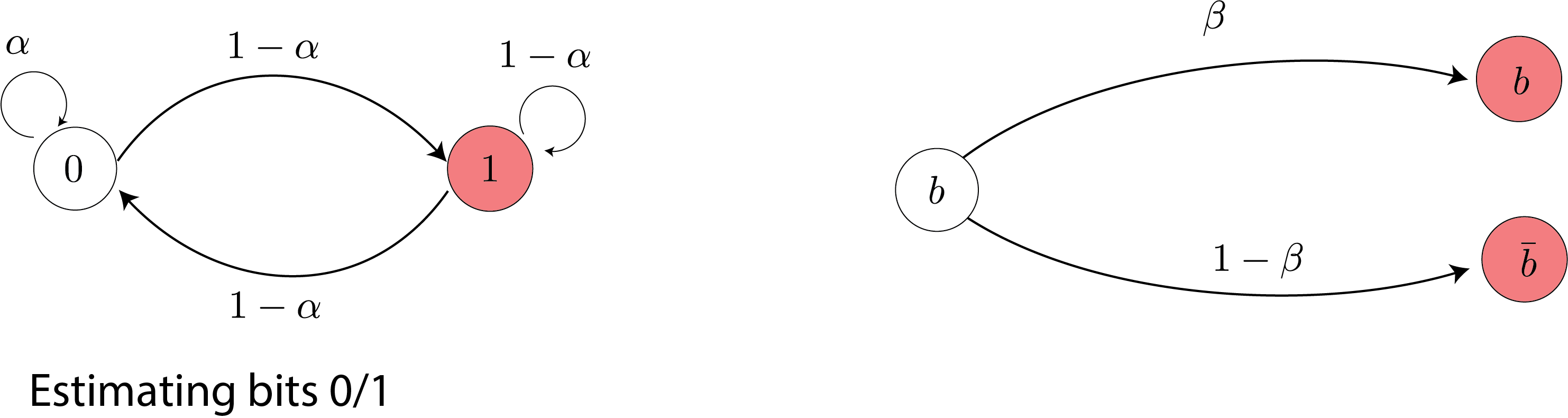
Here we only have two outputs, 0 and 1 (for example, in text, we have 27 results for all the characters in English).

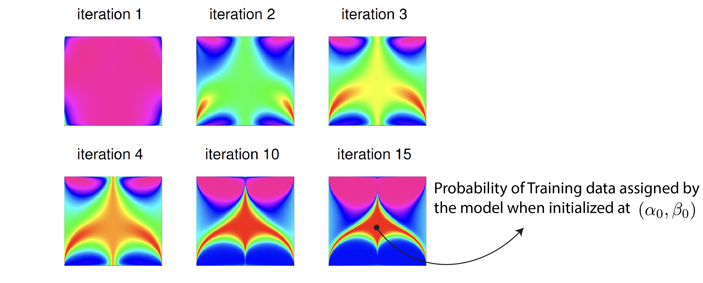
Takeaway point: training can be very sensitive to initialization.

Recurrent neural networks

After having a quick overview of recurrent neural networks, we will spend some time on recurrent neural networks, which can be thought of as a type of language model. They are similar to hidden Markov models, but the hidden layer is not stochastic. Instead, the transition is deterministic. The state is distributed (like embeddings), not definite, as for HMMs. We’ll describe this using characters rather than words — we could do either.

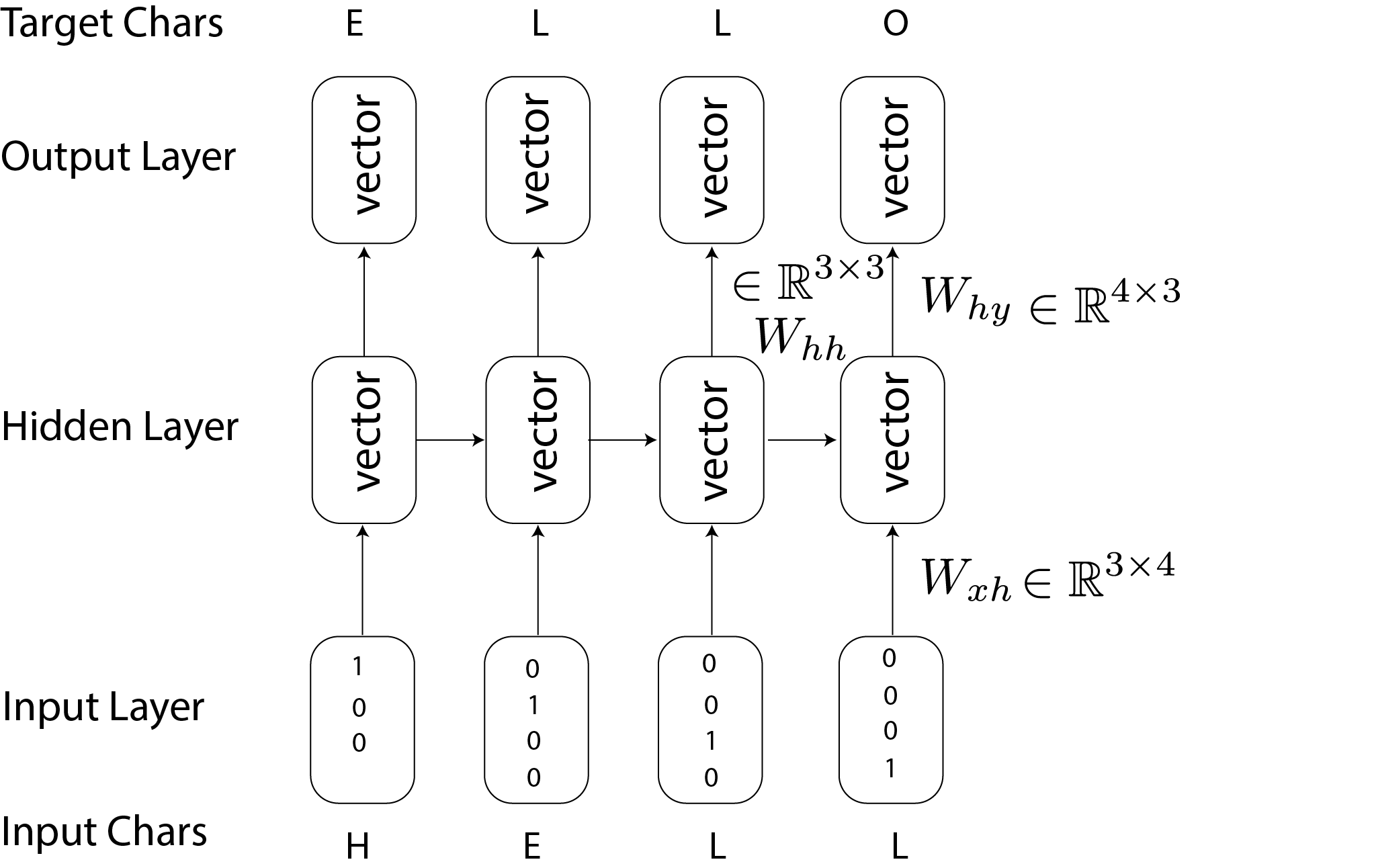
$$ \begin{align} h_t = & \text{tanh}(W_{hh}h_{t-1} +W_{xh} x_t) \\ y_t = & W_{hy} h_t \\ x_{t+1} | y_t \sim & \text{Multinomial}(\pi (y_t)) \end{align} $$

where $\pi(.)$ is the softmax function.

In this illusteration, $x_t$ is the “1-hot” representation of a character, $W_{xh}\in \mathbb{R}^{3\times 4}$, $W_{hh}\in \mathbb{R}^{3\times 3}$, and $W_{hy}\in \mathbb{R}^{4\times 3}$.

1
2
3
4
5

class RNN
    def step(self,x):
        self.h = np.tanh(np.dot(self.W_hh,self.h)+np.dot(self.W_xh,x))
        y = np.dot(self.W_{hy},self.h)
        return y

In a one-hidden-layer case:

1
2

rnn = RNN()
y = rnn.step(x)

In two hidden layer cases:

1
2

y1 = rnn1.step(x)
y2 = rnn2.step(y1)

Long short-term memory (LSTM)

A variant called “Long Short-Term Memory” RNN has a special hidden later that “includes” or “forgets” information from the past. Intuition: In language modeling, it may be helpful to remember/forget gender or number of the subject so that personal pronouns (“he.” vs.” she” vs." they") can be used appropriately. They are helpful for things like matching parentheses, etc.

A simpler alternative to the LSTM circuit is the Gated Recurrent Unit (GRU).

Each component is a tanh-thresholded linear function of the previous states and current input—a “neuron”.

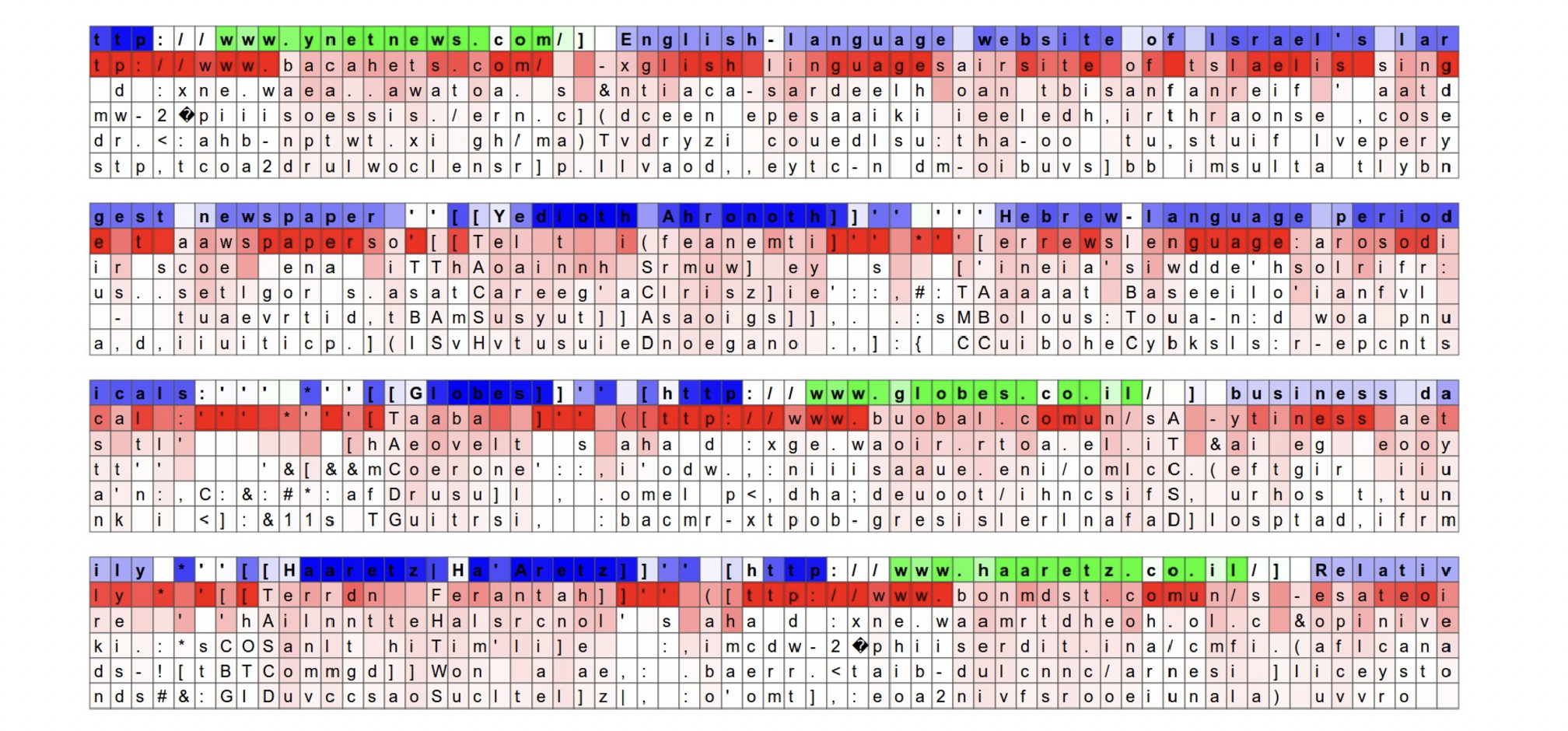
If the jth neuron $h_{tj}$ is close to $\pm 1$, it is very “excited.” This is colored green in the following illustration. If it is near zero, it is “not excited” or relaxed—colored blue.

Below the neuron color, the five most probable characters $c$ are shown — ordered in decreasing order of $y_{tc}$ and hence $\pi(y_{tc})$. Three layers, with 512 neurons on each level. Most will be completely uninterpretable. Recall—it’s generally hard to interpret coefficients in the least squares linear regression model!

The neuron highlighted in this image is very excited about URLs and turns off outside of the URLs. LSTM is expected to remember if it is inside a URL or not using this neuron.

Here, the highlighted neuron gets very excited when the RNN is inside [[]] markdown environment and turns off outside. Interestingly the neuron can’t turn on right after it sees the character [, it must wait for a second [ and then activate. This task (counting whether the model saw one or two open [) is likely done with a different neuron.

Vanilla RNN

In principle, the state $h_t$ can carry information from far in the past. But the problem is that the gradients vanish (or explode) in practice, so this doesn’t happen.

$$ \text{Loss} = - \log p(\text{next symbol}) $$

We want to predict the next symbol with high probability (i.e., equivalently minimizing the loss). To do that, we need to back-propagate the gradient through the layers of a neural network. We have to propagate this derivative back in time, for that neuron will balance parenthesis to do its job. The problem is the derivative becomes small and more minor and vanishes: it’s called vanishing gradients.

There is a complementary problem which is exploding gradients. It’s an easier problem because you can clip those gradients and chop them off. On the other hand, in a vanishing gradient, indeed, the signal disappears.

Instead, we need other mechanisms to “remember” information from far away and use it to predict future words.

Remember that in vanilla RNN state is updated according to the:

$$ h_t = \tanh (W_{hh}h_{t-1} +W_{xh} x_t+b_h) $$

We’ll modify this with two types of “neural circuits” for storing information to be used downstream. Both LSTMs and GRUs have longer-range dependencies than vanilla RNNs. We’ll go through this in detail for GRUs, which are more straightforward, more efficient, and more commonly used.

We’ll need to use pointwise products. This is given the fancy name “Hadamard product” and wrote:

Learn when to update the hidden state to “remember” important pieces of information, for example until seeing the closed ]. Or keep the fact that a word is plural and keep this in mind until reaching a verb. And use this information for number agreement between the subject and the verb. Could you keep them in memory until they are used? Reset or “forget” this information when no longer valid.

We will start with a simplified version of GRUs. We’ll make use of an update “gate” $\Gamma_t^u$. This is either zero or one. If $\Gamma_t^u=1$, we store/update information in a memory cell $c_t$. If $\Gamma_t^u=0$, we keep the information in the cell; don’t update it.

The memory cell using this simplified idea evolves according to: $$ c_t = (1-\Gamma_t^u) \odot c_{t-1} + \Gamma_t^u \odot h_t $$

Where $h_t$ is the state computed using the usual vanilla RNN. If the gate is 1, I am going to update the cell with the current state of RNN. If the gate is 0, I will carry over the memory cell from the last time. We predict the following words using the memory cell $c_t$ together with the usual RNN state $h_t$.

Everything needs to be differentiable, so the gate is “soft” and between zero and one.

Out equations are then: $$ \begin{align} \Gamma_t^U = & \sigma(W_{ux}x_t + W_{uh}h_{t-1} + b_u) \\ h_t = & \tanh (W_{hx}x_t +W_{hh}h_{t-1} +b_n) \\ c_t = & (1-\Gamma_t^u ) \odot c_{t-1} + \Gamma_t^u \odot h_t \end{align} $$

We predict the following words using the memory cell $c_t$ together with the normal RNN state $h_t$.

Remember:

$$ \begin{align} \sigma(x) = \text{sigmoid}(x) = & \frac{1}{1+e^{-x}} \\ =& \frac{e^x}{1+e^x} \end{align} $$

Example:

$^1$ The flowers $^2$, even though it was still so cold outside in New Haven, bloom in April

1. subject: The flowers
2. verb: bloomed
3. semantic components between bloom and April and also between flowers and April

We want to remember flowers even though it’s far from blooming and April. In location $^1$, $\Gamma_u=0$, we want to keep whatever is in the memory up to that point. In location $^2$, $\Gamma_u=1$ and we want to update the memory and put flowers in the memory. In location $^3$, $\Gamma_u=0$ and we want to keep flowers in the memory. In the next positions $^4$, $^5$, and etc $\Gamma_u=0$.

Before reaching bloom $\Gamma$ is close to 0, the gradient doesn’t vanish. So in backpropagation, there is enough juice in that gradient to learn this.

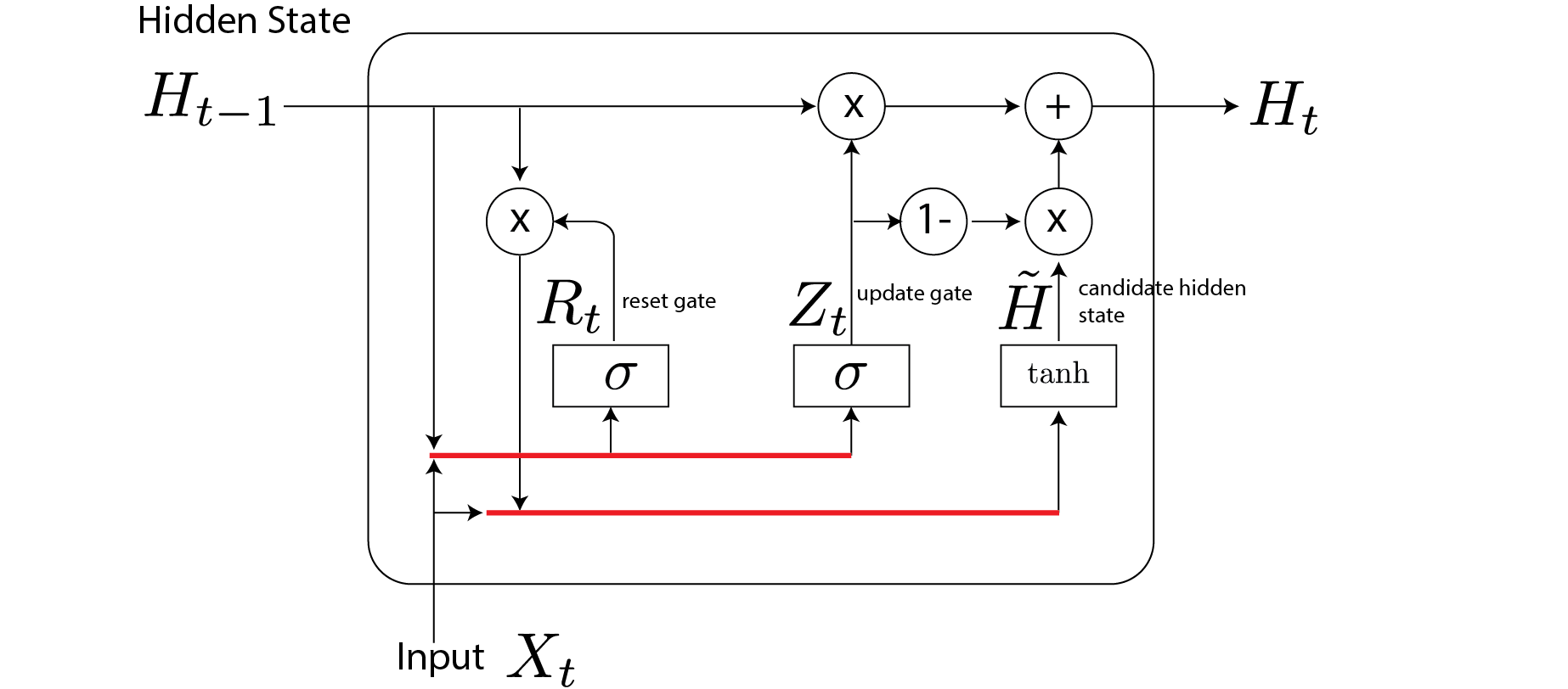
GRUs

This version uses two gates. One gate $\Gamma^u$ to update the memory cell. Another gate $\Gamma^r$ to decide if the state should be “reset”:

$$ \begin{align} \Gamma_t^U = & \sigma(W_{ux}x_t + W_{uh}h_{t-1} + b_u) \\ \Gamma_t^r = & \sigma(W_{rx}x_t + W_{rh}h_{t-1} + b_r) \\ h_t = & \tanh (W_{hx}x_t +W_{hh}(\Gamma_t^r \odot h_{t-1}) +b_n) \\ c_t = & (1-\Gamma_t^u ) \odot c_{t-1} + \Gamma_t^u \odot h_t \end{align} $$

$(\Gamma_t^r \odot h_{t-1})$ is the part that reset the memory. Other parts are similar to RNN.

LSTMs

A variant called “Long Short-Term Memory” RNN has a special context/hidden layer that “includes” or “forgets” information from the past.

$$ \begin{align} \text{forget: } F_t = & \sigma(W_{fh}h_{t-1} + W_{fx}x_{t} + b_f) \\ \text{include: } I_t = & \sigma(W_{ih}h_{t-1} + W_{ix}x_{t} + b_i) \end{align} $$

“Memory cell” or “context” $c_t$ evolves according to:

$$ \begin{align} c_t = & F_t \odot c_{t-1} + I_t \odot \tilde{c_t} \\ \tilde{c_t} = & \text{tanh} (W_{ch}h_{t-1}+W_{cx}x_t+ b_c) \end{align} $$

where $\tilde{c_t}$ is the updated cell.

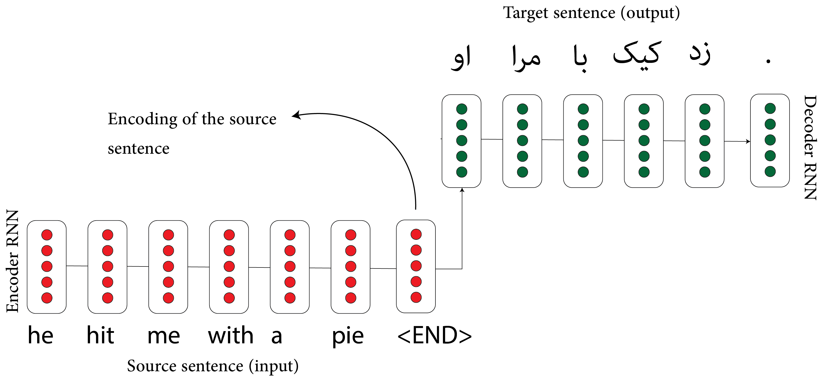
Sequence to Sequence models

Important in translation. Uses two RNNs (GRUs or LSTMs): Encoder and Decoder:

When you start thinking about this, everything looks like a sequence-to-sequence problem: text summarization and speech recognition. A traditional approach uses the Bayes theorem: from a text to an acoustic signal from a probabilistic/language model. But, using the seq to seq model, which APIs like Siri usually use, they directly map acoustic to text.

What we want is a conditional model of the target language/text given the input text:

$$ p(y_1,..,y_T| x_1,..,x_s) $$

We want this probability. The way we do that is just as what we did for an RNN, we factor it as a product of conditional probabilities:

$$ \prod_{t=1}^T p(y_t | h,y_1,..,y_{t-1}) $$

This resulted in a “bottleneck” problem as you push all the information from the English sentence to these neurons.

Question: If we wanted to model this using HMM, how would we change this? Answer: It should be sum or mixture model: $\sum_{t=1}^T \phi_i p(s_t | h,s_{t-1})$. However, models like GPT3 don’t use these latent variable models, which could be computationally more efficient.

We are dependent on the encoding of the source sentence to translate the sentence.

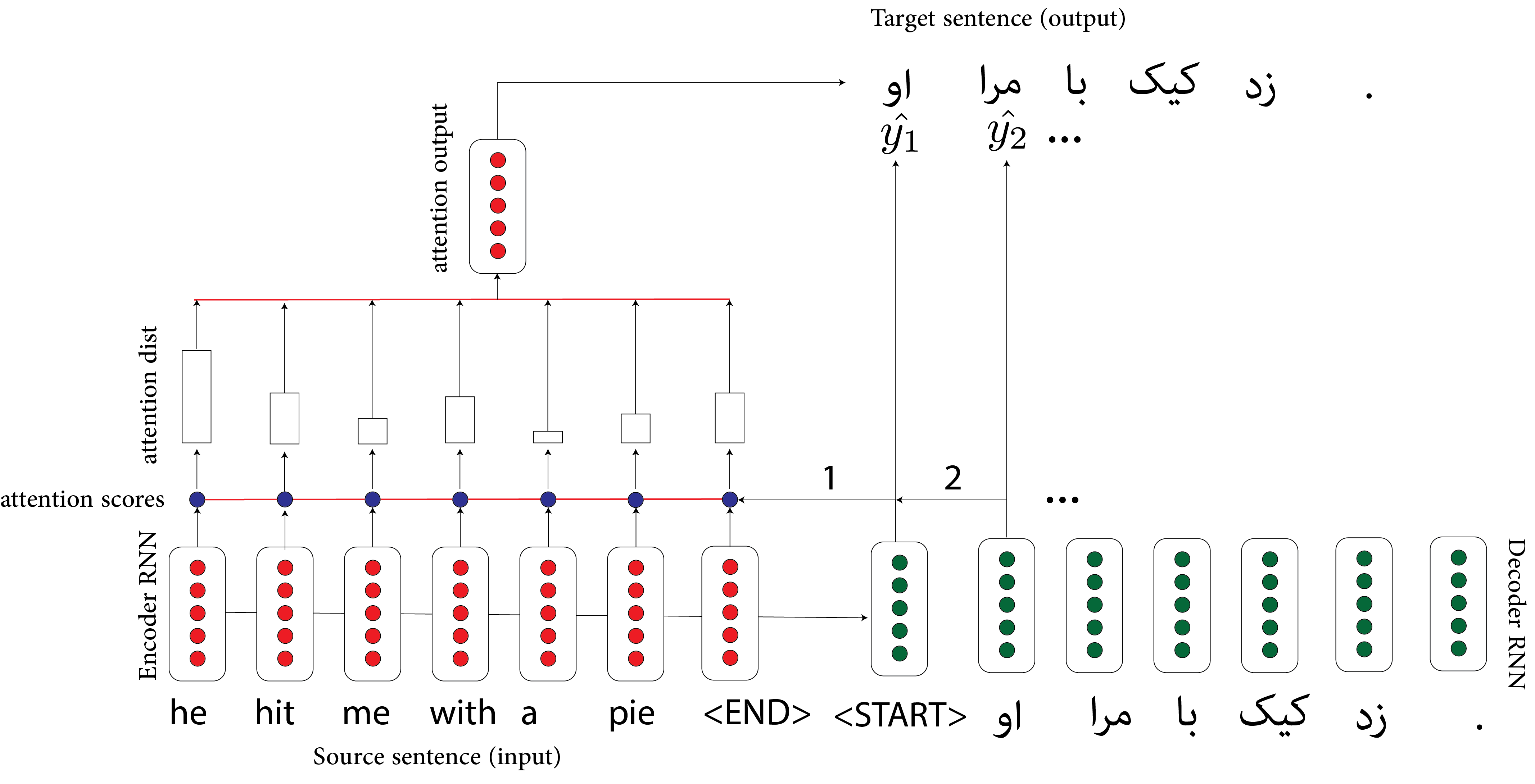
Necessary modification: use Attention. On each decoding step, directly connect to the encoder, and focus on a particular part of the source sequence. Indeed, those words are important in the source language and the given sentence.

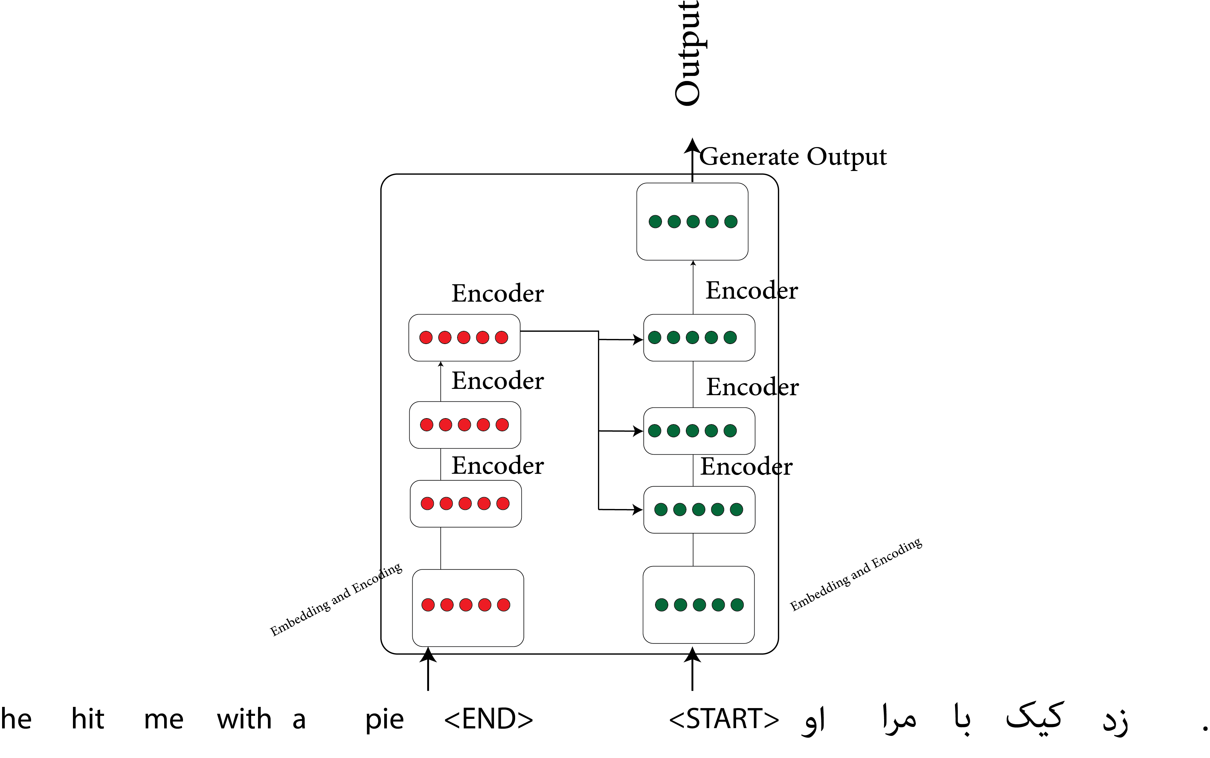
Transformers

The current state-of-the-art is based on transformers. Attention is the key ingredient. Rather than processing sequences word-by-word, transformers handle more significant chunks of text at once. The distance between words matters less.

Remember kernel density estimation, which is a close concept to kernel regression:

$$ f(x) = \frac{1}{n} \sum_{x_i \in D} K_w(x_i,x) $$

In kernel regression:

\begin{align} m(x) =& \sum_{i=1}^n \frac{K(x_i,x)Y_i}{K(x_i,x)} \\ =& \sum_i \alpha_i x \end{align}

where $\sum_i \alpha_i = 1$. These $\alpha_i$ s are like attention variables. We have all our data $x_1,..,x_n$, and we want to predict $x$ by assigning weights/vectors to data. Indeed, like the attention mechanism, $K(.,.)$ is the probability distribution that assigns the weights.

The transformer is based on an attention mechanism, and the main idea is to eliminate the sequences of RNNs.

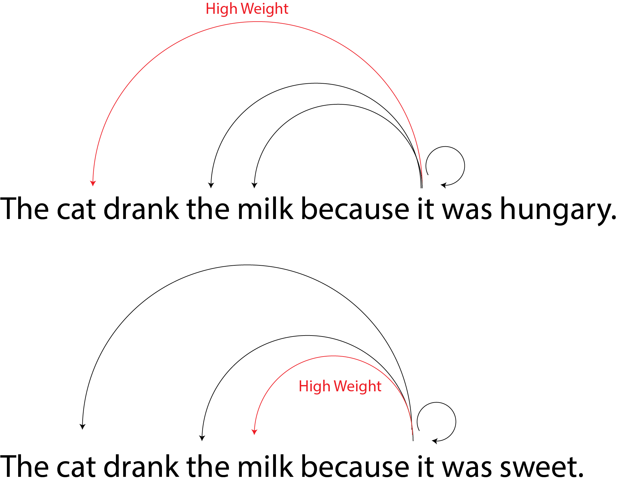
Two examples:

Sometimes people call this self-attention.

We covered this post in the intermediate machine learning SDS 365/565, Yale University, John Lafferty, where I was TF.